Chicago Open Rideshare Dataset - Getting Started

How to get started with mapping GIS data

29 Apr 2019

Introduction

I was recently reading Steve Vance and John Greenfield’s article summarizing data from the City of Chicago’s publishing of anonymized ride hailing data, and decided to look into the dataset on my own. The data shows all trips on Uber, Lyft, and Via from 11/1/2018 through 12/31/2018, starting and/or ending in the City of Chicago. The data includes the below for each rideshare trip:

Pickup census tract
Dropoff census tract
Total trip time elapsed
Trip distance
Fare paid
Tip paid
Whether the trip was a “shared” ride (e.g., UberPool)
Trip start and end time, rounded to the nearest 15 minutes

There are 17 million+ trips reported.

I figured I would play around with the data, to at least learn some new skills, and at most find something interesting in the dataset. I also wanted to share with others how I went about the technical aspects of my exploration.

Results

Disclaimer: For many of the trips, the pickup and/or dropoff census tract is omitted from the dataset. This is either due to the trip starting/ending outside of the city, or the city electing to anonymize that trip due to privacy concerns (some census tracts are very small and you might be able to identify an individual person from the public data). I ignored trips without a census tract, which skews the results below. There are potentially other data cleaning issues - this post is intended to be more educational on how to produce these maps, as opposed to finding anything particularly interesting in the data

My first idea was to simply look at the raw number of trips, by pickup location:

Number of trips by pickup location:

Take a look at the logarithmic scale in the legend. It’s hard to pick a proper color gradient for a map… But some of the numbers are much lower than I expected. Keep in mind the dataset includes all trips on Uber, Lyft, and Via from 11/1/2018 through 12/31/2018.

Number of trips by dropoff location:

This seems basically the same as the pickup map.

Next, I figured it would be fun to see where people are tipping more per mile. I figured tip per mile traveled is a good proxy for “cheapness”, although maybe dividing by the median household income of each dropoff tract would be even more interesting.

Tip per mile traveled, by dropoff location:

While I think there’s a lot more I can do with the dataset, I’ve spent a lot of time on this post so I’m going to stop here for now. My main motivation was to learn how to play with GIS data and visualize it on the web, and I think I accomplished that. I hope someone else can learn something from the very detailed walkthrough below.

How Did I Do This?

I did some research, and found that PostGIS is a very popular, open-source Postgres extension for dealing with GIS data. Postgres is a relational SQL database, but doesn’t have any GIS capabilities out of the box. I had used Postgres before. Postgres can help us answer questions like “Which census tract paid the most in tips?”. I also wanted to use Leaflet, a JavaScript library that is used for map visualizations, in order to visualize some of our findings.

So, the plan looked something like this:

Set up Postgres database with PostGIS extension
Import all 17 million trips into the database
Query the dataset for some interesting finding
Map the finding using Leaflet, so we can see our results in a pretty webpage

If this means nothing to you, then great! I’ll provide plently of detail below. If it’s too much detail, don’t worry, hopefully I’ll have more interesting findings in future posts.

This post should hopefully be comprehensible by people with minimal computer experience.

The Details

A wise man once told me, “the devil is in the details”

Digital Ocean

It will probably be easiest if you use the exact same setup as me, so I think it’s best that you get a “droplet” set up on Digital Ocean. A droplet is just a virtual machine (basically a server) that you can get in the “cloud”. Oooooh. Heard of the cloud before? It’s a beautiful, white, fluffy place. Once you create an account, you will be able to get a server with lots of resources (don’t worry, we’ll use one with very few resources) in a matter of seconds. I like Digital Ocean for its simple interface and simple pricing. With AWS I often struggle to understand how much I’ll be paying. Using a server will be nice to make sure we don’t ruin our own personal machines, and also to have enough hard disk space (the dataset is big). Also, the $5 monthly fee is pro-rated, so if you finish this demo in a few hours, you’ll be paying pennies.

If you don’t want to pay anything, you are more than welcome to get Postgres set up on your own machine. You’ll just have to look elsewhere on the web for instructions for this part of the post.

Once you create your account, you’ll want to create a new droplet by clicking on “Create” in the top right of the dashboard:

Then choose Ubuntu 16.0.4, Standard plan. These should be the default.

droplet-1

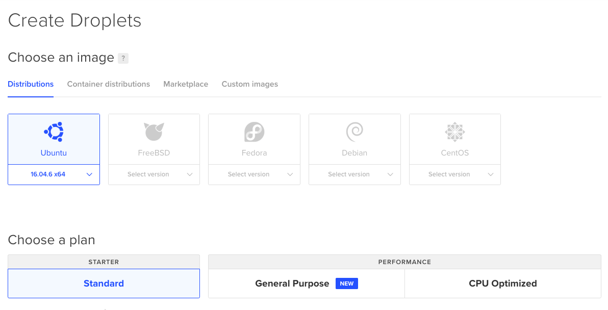
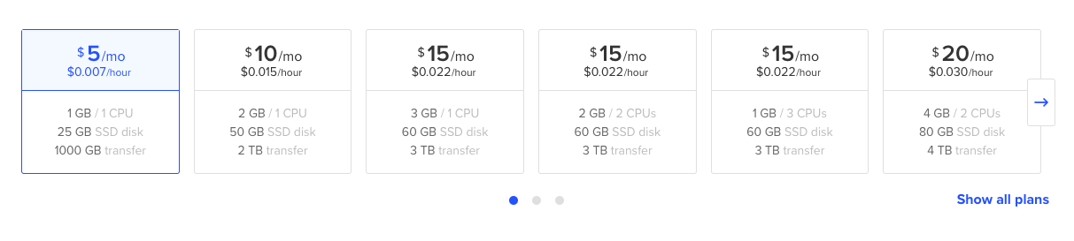
Be sure to get the cheapest droplet, at $5 a month. To reiterate, this is pro-rated and you can very easily destroy a droplet and close out your account.

5-dollar

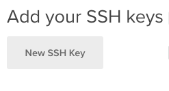
Now, for the important part. Add a new ssh key:

new-ssh

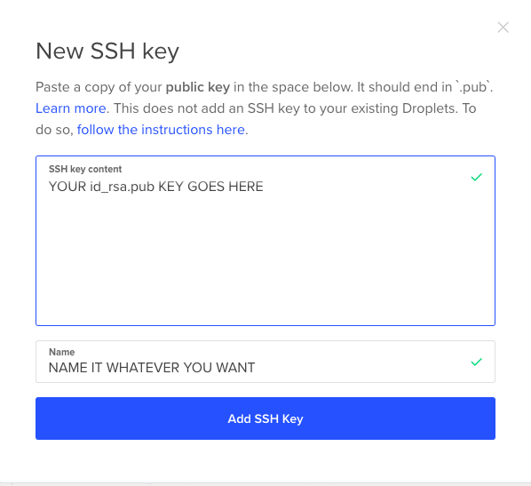
Now, we need to generate an ssh key on our local machine. Ssh stands for “secure shell”, and is a secure way to remotely access a server. We need to generate the a secure key that we’ll give to Digital Ocean, so that when we try to login to our server, Digital Ocean will know that we’re authorized to access the machine. To generate an ssh key, open up your Terminal application (I’m on OS X, but if you’re on Windows, open up Git bash instead of the normal Windows command prompt). Type ssh-keygen, and hit enter to use all the defaults. Next, type cat ~/.ssh/id_rsa.pub. You should see a bunch of letters that mean nothing to you. Go ahead and copy this entire string into Digital Ocean.

add-ssh

Now, create the droplet and head back to the Digital Ocean dashboard. You should see your droplet and its IP address in the Dashboard.

dashboard-ip

Now in your Terminal, run ssh root@<IP ADDRESS HERE>. So I’ll run ssh root@206.189.194.182. You should be logged on to the server now.

Postgres

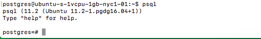
Let’s download Postgres. Type vim /etc/apt/sources.list.d/pgdg.list. vim is a Terminal-based text editor. When you open it, you start out in “normal” mode. In normal mode, you can’t type anything. So hit i to enter insert mode, and type deb http://apt.postgresql.org/pub/repos/apt/ xenial-pgdg main. Then hit the escape key, and type :wq and then Enter to exit vim and save the changes to the file. By adding this to the file, we’re enabling the program apt to download Postgres for us from this repository. apt comes with certain Linux distributions, and is a really handy way to download programs. Also, run wget --quiet -O - https://www.postgresql.org/media/keys/ACCC4CF8.asc | apt-key add -. Then, simply run apt-get update in order to pull in this new repository. Then, run apt-get install postgis. Then, run sudo su - postgres to change the user you’re currently running as from root to the user named postgres, which should have been automatically created when you install PostGIS and Postgres. Then, run psql.

If this all worked, you should now be logged in to a Postgres database instance. It should look like the below picture. If so, congrats! We’re almost ready to make really cool maps and stuffs.

postgres-initial

When you log in to the Postgres server, you’re initially put in a default database called “postgres”. Let’s make our own database to store the rideshare data:

CREATE DATABASE rideshare;

Then, let’s change to this database:

\c rideshare

You should see psql say something like You are now connected to database "rideshare" as user "postgres"..

Now, let’s create a user that can login to the database:

CREATE USER rideshare WITH PASSWORD 'rideshare';

Then, since we don’t really care about security, let’s make this user with a very easily-guessable password the owner of our new rideshare database:

ALTER DATABASE rideshare OWNER TO rideshare;

Now, if we login as user “rideshare”, with password “rideshare”, we can do anything in the “rideshare” database. Now, let’s install PostGIS to let us store and query geographic data:

CREATE EXTENSION postgis;
CREATE EXTENSION postgis_topology;

Now, let’s create a table to store all the trip data. I’ll call it “trip”. A table is more or less an Excel sheet but in database world. Wow this is getting exciting.

CREATE TABLE trip (
	trip_id char(40) UNIQUE,
	trip_start_timestamp timestamp NOT NULL,
	trip_end_timestamp timestamp NOT NULL,
	trip_seconds int NOT NULL,
	trip_miles numeric(8, 1) NOT NULL,
	pickup_census_tract bigint,
	dropoff_census_tract bigint,
	fare numeric(8, 2) NOT NULL,
	tip smallint NOT NULL,
	additional_charges numeric(8, 2),
	shared_trip_authorized boolean NOT NULL,
	trips_pooled smallint NOT NULL,
	pickup_centroid_location geometry(POINT, 4326),
	dropoff_centroid_location geometry(POINT, 4326)
);

These columns align 1-to-1 with the columns in the dataset. Notice the last two columns are of type geometry(POINT, 4326). This datatype is provided to us by the PostGIS extension that we installed. If you’re at the point in the blog post where you’re ready to start browsing through an incredible amount of unrelated web pages, this is your chance. Let me get you started. 4326 is the European Petroleum Survey Group (EPSG) code for the World Geodetic System (used in GPS). The EPSG no longer exists, it was merged into the International Association of Oil & Gas Producers, but the EPSG acronym stuck. You’re probably most familiar with EPSG 4326 even if you’ve never heard of it. It’s basically lat/lon. So since the City of Chicago gives us the data in lat/lon, we’ll import it as such. There are two types of columns in PostGIS, geometry and geography. Geography handles issues with arcs (the world isn’t flat), but is slower and less feature-rich. Since our data points are very close together, these curved-earth issues shouldn’t matter to us. I personally still cannot understand how inputting data as 4326 but storing it as a geometry makes any sense, but we’ll do it anyway for now. My understanding was that geometries had to be projected data. But maybe gometry(4326) is an unprojected projection? If you’re reading this and have any input on this, please leave a comment!

I found this post by Lyzi Diamond from Mapbox quite useful. It explains the differences between the two most common EPSG projections for the web, 4326 and 3857. If you don’t read that article, at least watch this video from the West Wing. It’s fantastic.

Now, we need to download the data from the City of Chicago website, and get it into this darned database. We’ll need to do some small tranformations on the data downloaded from the City in order to import it. Python is a great scripting language perfect for this task.

Let’s exit out of psql by running \q. We should now be back in our normal ssh terminal. Let’s type exit again, so that instead of being logged in as the postgres user, we’re logged in as root. You should see something like the below:

root

apt-get install python-dev will install Python for us. Also run apt install virtualenv. virtualenv is a Python tool that helps us manage packages. We don’t want to write the code to insert data into Postgres ourselves, so we’ll install a package to do it for us. That package is called pyscopg2. First, create a Python virtual environment called rideshare_env. Run virtualenv rideshare_env to do so. Then, run source rideshare_env/bin/activate to “activate” the virtual environment, and install pyscopg2 by running pip install psycopg2-binary.

Ok folks, I can tell the anticipation is building. It’s time to import 17 MILLION rows of data into our database.

Run wget -O tripdata.csv https://data.cityofchicago.org/api/views/m6dm-c72p/rows.csv?accessType=DOWNLOAD to download the dataset into a csv. This might take a while… (took me about 20 minutes)

Now, for the slowest, most exciting part of our journey together. Getting the data into Postgres. Take a look at the Python script I wrote. You can download it by running wget -O import_rows.py https://raw.githubusercontent.com/samc1213/chicago-rideshare/master/import_rows.py. Make sure the rideshare_env environment is still activated (it will show up in the terminal prompt). Then run the script using python import_rows.py. If it’s working, it will print every 1000 rows that it imports. Yes, it has to get to 17 million, so go for a run, or grab a nice juicy cheeseburger once you see the script get started. This part took me about an hour.

Data Extraction

This is actually the fun part now. We need to get the data out of the database and into a gorgeous map that we can hang on the wall. I’m not creative, so the first thing I thought to look at was tipping. I wanted to map the ratio of tip to trip distance by dropoff census tract.

We’ll use a toolchain called GDAL to run queries on the Postgres database, and return the result of the query in a format called GeoJSON. The specific tool to do this is called ogr2ogr. It also works in the reverse direction. That is, given a GeoJSON file, it can import data into Postgres for us. This feature will be nice, since our dataset currently only contains dropoff_centroid_locations. We really want the entire geometry of the census tract in order to map the results nicely. Thankfully, the City of Chicago provides a nice GeoJSON file that gives the geometries of every census tract in Chicago.

First, run sudo apt install gdal-bin to install the GDAL tools. Then, download the City’s census tract dataset:

wget -O censustracts.geojson "https://data.cityofchicago.org/api/geospatial/5jrd-6zik?method=export&format=GeoJSON"

Then, use the new GDAL tool to import the data:

ogr2ogr -f "PostgreSQL" PG:"dbname=rideshare user=rideshare password=rideshare host=localhost port=5432" censustracts.geojson

Log back in to the database using psql --dbname=rideshare --host=localhost --port=5432 --username=rideshare (top-secret password is “rideshare”, don’t forget it), and run \d

gdal-census-import

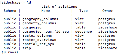
We see that the tool seemed to create a table called ogrgeojson for us. Let’s learn what’s in that by running \d ogrgeojson:

orgr-table

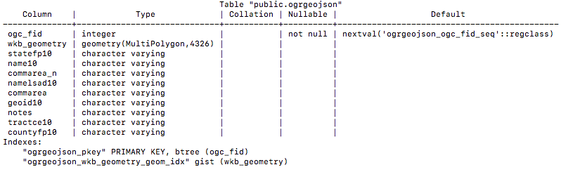
We can also run SELECT * FROM ogrgeojson LIMIT 1; to see an example of what’s in the table. Looks like the column geoid10 maps to the dropoff_census_tract and pickup_census_tract column from the rideshare database. Also, looks like the wkb_geometry column has the ST_MultiPolygon that draws out for us the boundaries of the tract (SELECT ST_geometrytype(wkb_geometry) FROM ogrgeojson; shows that). Great! So we can combine this census tract data with the rideshare data to make a pretty map. I personally hate the table name ogrgeojson. Plus some of the data in there is unneeded. Let’s make our own table with a nice name and clean data:

CREATE TABLE census_tract (
	census_tract_id bigint UNIQUE,
	tract_name varchar(50),
	tract_geometry geometry(multipolygon, 4326)
);
INSERT INTO census_tract SELECT cast(geoid10 as bigint), name10, wkb_geometry FROM ogrgeojson;

Now, let’s make a table to temporarily store the data we need for our pretty map. This will just have the data by dropoff_census_tract, which is just an id. We’ll have to combine this with the census_tract data to get the whole geometry of the census tract itself.

CREATE TABLE tip_by_tract AS
SELECT dropoff_census_tract, avg(tip/t.fare)
FROM trip t
WHERE t.fare != 0 GROUP BY dropoff_census_tract;

This query might take a little while. We’ve got 17,000,000 unindexed rows to go through. Took me a minute or two.

Now, lets make sure the data in the tip_by_tract table maps up to the census_tract data nicely. We’ll use a JOIN for this. If you’re new to SQL, you might want to read up on JOINs. I like to think of a join like this: Take the Cartesian product of all of the rows in each of the two tables you are joining (in our case, tip_by_tract and census_tract). Then, evaluate the ON clause for each of the pairs of rows (c.census_tract_id=t.dropoff_census_tract). If the ON clause is true, then return that row in the result. Otherwise, throw it out.

SELECT *
FROM tip_by_tract t
JOIN census_tract c
ON c.census_tract_id=t.dropoff_census_tract;

This seems to work fine, but it’s hard to look at in psql. Let’s get it out into GeoJSON and view it in a map. Run \q to go back to the command line.

ogr2ogr -f "GeoJSON" tip_by_census_dropoff.geojson PG:"dbname=rideshare user=rideshare password=rideshare host=localhost port=5432" -sql "SELECT * FROM tip_by_tract t JOIN census_tract c ON c.census_tract_id=t.dropoff_census_tract;"

That will write the results of the query to a file called tip_by_census_dropoff.geojson. All we need to do is map this file. Type pwd to see what directory you’ve been working in this whole time. I’ve been in /root. We can open up a new terminal window on our local machine, and run scp root@206.189.194.182:/root/tip_by_census_dropoff.geojson .. You’ll want to sub in the IP address of your Digital Ocean server for mine. This will copy the geojson file to your local machine. Then, create a file called index.html in the same directory as the geojson file on your local machine. It should look something like this

 <head>
 <link rel="stylesheet" href="https://unpkg.com/leaflet@1.4.0/dist/leaflet.css" integrity="sha512-puBpdR0798OZvTTbP4A8Ix/l+A4dHDD0DGqYW6RQ+9jxkRFclaxxQb/SJAWZfWAkuyeQUytO7+7N4QKrDh+drA==" crossorigin=""/>
<script src="https://unpkg.com/leaflet@1.4.0/dist/leaflet.js" integrity="sha512-QVftwZFqvtRNi0ZyCtsznlKSWOStnDORoefr1enyq5mVL4tmKB3S/EnC3rRJcxCPavG10IcrVGSmPh6Qw5lwrg==" crossorigin=""></script>

</head>
<body>
	<div id="map" style="height:500px;"></div>
</body>
<script src="my-map.js"></script>

Then, create a new file called my-map.js in the same directory, and put the below into it:

var map = L.map('map').setView([41.881832, -87.623177], 12);

L.tileLayer('https://{s}.tile.openstreetmap.org/{z}/{x}/{y}.png', {
    attribution: '&copy; <a href="https://www.openstreetmap.org/copyright">OpenStreetMap</a> contributors'
}).addTo(map);

let data = `
<COPY PASTE THE WHOLE GEOJSON FILE HERE>
`;

var info = L.control();

info.onAdd = function (map) {
	this._div = L.DomUtil.create('div', 'info');
	this.update();
	return this._div;
};

info.update = function (props) {
	this._div.innerHTML =  (props ?
		'<h3>tip / trip length (miles)</h3><b>$' + props.avg + ' </b><br>Tract ' + props.tract_name
		: 'Hover over a census tract');
};

info.addTo(map);

function getColor(d) {
    return d > .07 ? '#800026' :
           d > .06 ? '#BD0026' :
           d > .05 ? '#E31A1C' :
           d > .04 ? '#FC4E2A' :
           d > .03 ? '#FD8D3C' :
           d > .02 ? '#FEB24C' :
           d > .01 ? '#FED976' :
                      '#FFEDA0';
}

function style(feature) {
    return {
        fillColor: getColor(feature.properties.avg),
        weight: 2,
        opacity: 1,
        color: 'white',
        dashArray: '3',
        fillOpacity: 0.7
    };
}

var geojson;

function highlightFeature(e) {
    var layer = e.target;

    layer.setStyle({
        weight: 5,
        color: '#666',
        dashArray: '',
        fillOpacity: 0.7
    });

    if (!L.Browser.ie && !L.Browser.opera && !L.Browser.edge) {
        layer.bringToFront();
    }

    info.update(layer.feature.properties);
}

function resetHighlight(e) {
    geojson.resetStyle(e.target);
    info.update();
}

function onEachFeature(feature, layer) {
    layer.on({
        mouseover: highlightFeature,
        mouseout: resetHighlight,
        click: highlightFeature
    });
}

geojson = L.geoJson(JSON.parse(data), {
    style: style,
    onEachFeature: onEachFeature
}).addTo(map);

When you open up index.html in your browser, you should see something that looks like the maps at the beginning the post.

Beautiful, isn’t it? If this didn’t work for you, check out my small Github repo that contains the demo.

Next Steps

I’m honestly not that satisfied with these results from an analytical perspective. If you have any ideas of things to look at in the dataset, please leave a comment below. With this framework set up, it should be much easier to do additional analysis. I plan on following up with more maps and analyses in future posts.

Sam Blogs